Background

The influence of thermosphere neutral winds on the ionosphere is critical to understanding ionospheric dynamics. While the measurements of many of the properties of the ionosphere can be made reliably using radio propagation, radar techniques, and optical techniques, measurements of the properties of the neutral thermosphere are difficult. Measurements of upper atmospheric neutral air motion are required for any in-depth study of ionosphere-thermosphere coupling. The neutral winds affect many of the observable quantities and physical processes of the ionosphere, including the density profiles of the ionospheric F region and the generation and maintenance of electric fields. The behavior of neutral winds is one of the most important but poorly known factors affecting the day-to-day variations in ionospheric electron and ion densities because it controls the whole electron density profile by altering the rate at which the ions diffuse along magnetic field lines. Accurate quantitative modeling of F region densities is not possible without an accurate specification of neutral winds in the thermosphere. In addition, general circulation models need neutral wind data for validation.

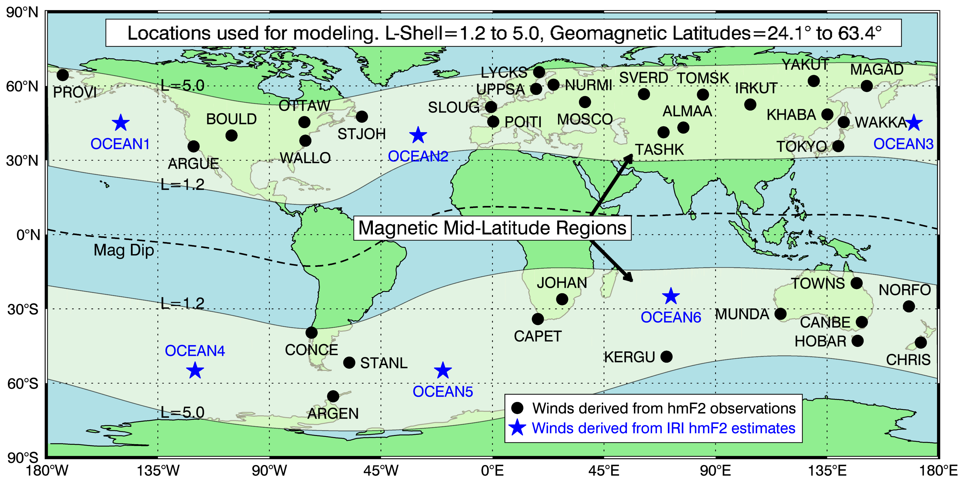
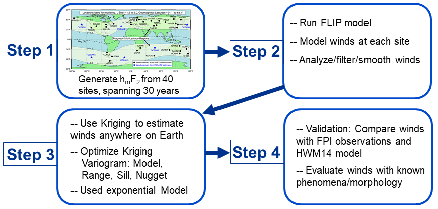
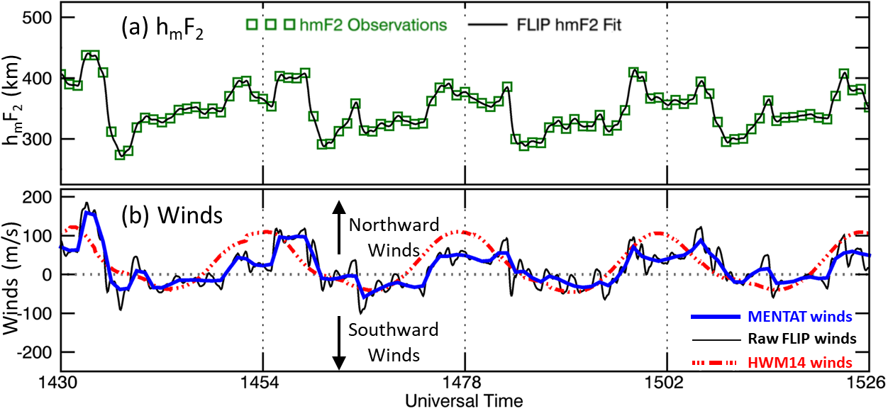
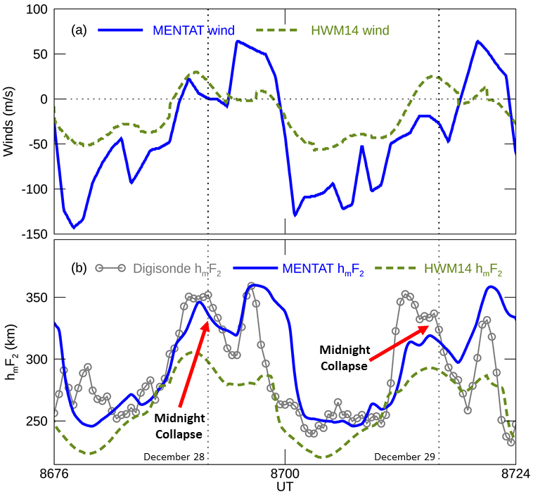
This research employs a method to derive the magnetic meridional component of equivalent neutral winds in the thermosphere from values of hmF2 derived from ionosonde measurements. The winds obtained from hmF2 are termed 'equivalent' or 'effective' neutral winds because they comprise both neutral wind and electric field contributions to changes in hmF2. The method has been shown to produce winds with comparable accuracy to other techniques and it has the advantage of being able to obtain winds both day and night and at the many mid-latitude ionosonde sites. The numerical technique has been developed over the past 20 years. The technique makes use of the Field Line Interhemispheric Plasma (FLIP) model of the ionosphere, which is a well-regarded first-principles model of the ionosphere and plasmasphere. The findings of this research provide an improved understanding of thermospheric winds and the resulting empirical wind model will be a useful tool for ionospheric researchers.

Empirical Modeling

How Horizontal Winds in the Thermosphere Affect the Ionosphere

Due to drag forces (known as ion drag) between the neutral particles in Earth's thermosphere and charged particles in Earth's ionosphere (the ionospheric plasma), neutral atmospheric winds may force the ionospheric plasma to move along with it.
However, the charged particles are constrained to move parallel to Earth's magnetic field lines... which means that the charged particles (the ionospheric plasma) will move both horizontally and vertically.
The result is that the plasma may be forced upward (or downward) in altitude, depending on the direction of the winds and the angle of Earth's magnetic field lines where a wind is occurring.
The animation below shows the effect of Southward winds in the Northern hemisphere, which are driving a local ionospheric plasma up Earth's magnetic field lines. Please note that this cartoon does not address all of the relevant physics... it is simply meant to demonstrate the effect of neutral winds on an ionospheric plasma in the thermosphere. For details, please read the PHYSICS NOTE located just below the animation.

Animation of effect of Southward winds in the Northern hemisphere

PHYSICS NOTE: Near and above the F2 peak below ~450km, O+ ions normally diffuse downward under gravity both day and night. During the daytime, poleward winds act to enhance the downward O+ motion. This increases the electron density at lower altitudes causing hmF2 to decrease. Nighttime equatorward winds (the above animation) generally act to retard the downward motion of the O+ ions , which keeps ions at higher altitudes where loss rates are slower, causing hmF2 to increase.

Locations that were used to Model the Neutral Winds

The map below shows the 40 locations that were used to develop this new empirical wind model.
All of the locations are located in the magnetic mid-latitude regions, which span Earth's magnetic L-Shells from L=1.2 to L=5.0. The magnetic mid-latitude regions are indicated on the map by the light-yellow bands in the northern and southern hemispheres.
The local vertical inclination of Earth's magnetic field (dip) ranges from -35.7° at Concepción, Chile (CONCE, in South America) to +73.6° at Provideniya, Russia (PROVI, top/left on map).

Map showing 40 locations that were used to develop this new empirical wind model

Modeling Technique & Formulation

The four top-level stages for developing the wind model are shown below. They include calculating the ionospheric altitude heights (hmF2 values) from hand-scaled ionospheric parameters, running the modified FLIP model to generate the magnetic-meridional neutral winds, using Kriging to generate hourly/global wind maps, building the new empirical model, and then validating the model against ground-truth wind observations and known/expected wind behavior.
There were also many additional underlying steps required to develop the model. For example, optimizing the FLIP model runs to regularly generate physically-realistic winds at each location took a very long time. Determining the best semivariogram function and parameters for the geostatistical Kriging interpolation was very involved. The modeled winds at each site had to be evaluated for biases and 'strange' behavior. And then, finally, packaging the algorithms into a smart/fast easy-to-use software package had to be done.

Using Kriging to Generate Global Wind Maps

A special type of interpolation, known as Kriging, was used to build global hourly wind maps from the derived winds at the 40 locations shown above, using an exponential semivariogram model.
Winds were only derived in the mid-latitude regions, but they were interpolated to span the polar and equatorial regions. There are very strong dynamics in those regions which also drive the neutral winds, but it will be interesting to see how the MENTAT winds perform in those regions - especially during periods with low geomagnetic activity.

Diagram showing wind pattern activity before and after Kriging

General Wind Morphology

Hourly Winds

The image below shows observations and modeled values at Canberra, during March 1-5, 1990. Plot (a) shows hourly ionosonde hmF2 observations (green squares) and the FLIP model fit to the observations (solid black line). Plot (b) shows the raw modeled FLIP equivalent winds (solid black line), MENTAT empirical model winds (thick blue line), and HWM14 winds (red dashed line). The vertical dotted line indicate midnight local time.
The FLIP model does a very good job of tracking the hmF2 observations.
The MENTAT winds in plot (a) exhibit the hourly surges and abatements that are required to reproduce the hmF2 observations seen in plot (b), while the HWM14 winds do not.

Diagram showing observation data from Canberra, during March 1-5, 1990

Global Winds

The image below shows global MENTAT and HWM14 winds for March 25, 1990, UT=19. HWM14 winds are shown in the upper wind map, and MENTAT winds are shown in the lower wind map.
The general behavior of global thermospheric winds is to flow from the dayside to the nightside. This is due to the larger temperature - and therefore pressure - on the dayside due to heating from the sun. On the plot below, Noon local time is shown as the yellow circle with 12PM in the center and Midnight local time is shown as the dark gray circle with 12AM in the center.
The MENTAT wind map shows the expected wind behavior: the winds flow from around 12 PM (noon) local time toward the antipodal location on Earth's nightside, around 12 AM (midnight) local time. The winds flow over the pole and gain speed along the way. On the HWM14 wind map, however, there are no winds flowing northward in the entire northern hemisphere.

Diagram showing global MENTAT and HWM14 winds for March 25, 1990

24-Hours of Global Winds

The animated GIF below compares 24 continuous hours of MENTAT and HWM14 winds, one hour at a time. It repeats over and over so that you can observed some differences between the two models.
The MENTAT diurnal winds behave as expected, but the HWM4 winds in the North American sector never flow northward during the entire 24-hour period. This is indicated in the red areas in both plots.

Animation showing 24 continuous hours of MENTAT and HWM14 winds, one hour at a time

Solar Flux Dependence

The amount of (non-storm-time) energy that our sun generates is not constant. Over an 11-year period, the level of output energy from the sun increases and decreases. This solar variability significantly affects the speed of neutral winds in the thermosphere.
One may reasonably imagine that, when the sun is producing more energy, the winds in the thermosphere will flow faster. However, due to the effects of ion drag, the opposite is actually true. When the sun is more active and putting more energy into Earth's atmosphere, more ions are being created, and the increased drag between the ionized and neutral particles is larger.
The level of solar energy input to the thermosphere increases by about a factor of 3 or more over the 11-year solar cycle, which increases the driving force for neutral winds. However, the solar cycle effect on the neutral wind speeds actually become smaller because of increased ion drag due to a factor of 3 or more increase in ion density.
In the plot below, this effect can be seen in the MENTAT winds: the annual median wind speed is largest during solar minimum (when F10.7A and NmF2 are low), and the median wind speed is lowest during solar maximum (when F10.7A and NmF2 are large).
The effect is not seen at all in the HWM14 model winds. This sensitivity to solar variability is a significant advantage of the MENTAT model winds.

Seasonal Bulk Flow of MENTAT Winds

The plot below shows the large-scale, north-south hemispheric wind flow of the MENTAT winds during a winter month and summer month every year from 1961 to 1990. Blue bars represent the net wind speed and direction during every January and red bars are for July. Winds were generated using 180 locations in the magnetic mid-latitudes, with 90 in the northern hemisphere and 90 in the southern hemisphere.
During summer in the northern hemisphere (July), the net wind flow should be southward.
During summer in the southern hemisphere (January), the net wind flow should be northward.
This analysis has not yet been done for HWM14 winds.

Plot showing the large-scale, north-south hemispheric wind flow of the MENTAT winds during winters and summers from 1961 to 1990

Validation: Comparison with FPI Observational Data

Comparison on one night with three FPIs

As a comparison with 'ground truth' observational data, MENTAT winds are compared to three Fabry-Pérot interferometers (FPI). The geographic location, local magnetic declination (BDEC), and local magnetic inclination (BINC) of each site is shown in the map and table below.

Map image showing geographic location, local magnetic declination (BDEC), and local magnetic inclination (BINC) of each site

A comparison of modeled winds with winds from the three FPI instruments is shown below. The figure shows the MENTAT and HWM14 winds, observed FPI winds, and Equivalent Winds at the three FPI sites on the night of March 23, 2014. Equivalent winds are the raw derived winds from the FLIP model that were used to create the MENTAT empirical model.
The horizontal dotted line in the wind plot denotes where the winds change direction from northward to southward. The FPI optical integration time for each FPI wind observation was 15 minutes. The FPI winds at the VTI and PAR locations differ significantly from the winds at UAO. The differences are attributed to the presence of clouds at UAO which pull the winds towards zero.
The MENTAT winds do not reproduce the FPI data quite as well as the Equivalent winds, but they generally match the FPI observations better than the HWM14 winds. The MENTAT winds reproduce the daily trend of the FPI wind data quite well at VTI and PAR locations. The MENTAT winds transition from northward to southward between 6:00 PM and 8:00 PM at each site, which is similar to the behavior of the FPI winds. The HWM14 wind speeds, on the other hand, do not change direction during that time period at any of the three locations.

Charts showing a comparison of modeled winds with winds from the three FPI instruments

Comparison with One FPI During Four Seasons in Year=2014

A seasonal comparison of modeled winds with FPI wind observations at the PAR location during four seasons in 2014 is shown below.
The FPI at PAR was chosen for this comparison because it had the most wind observations overall and the most wind observations in each 15-minute time interval. The spring period consists of 25 days of data, spanning March 22 to April 15 UT, 2014. The summer period consists of 29 days of data, spanning June 16 to July 14. The fall period consists of 30 days of data, spanning October 17 to November 15. The winter period consists of 31 days of data, spanning January 19 to February 18.
For each season in the plot below, the black dots with red error bars in the top frame show all the 15-minute FPI observations, and the solid black lines show the median FPI wind for that season. The center frame for each season display the raw modeled MENTAT winds for the season as overlapping lines and the median MENTAT wind is shown as the dashed black line. The lower frame for each season show the raw HWM14 winds (blue lines) and the median HWM14 wind is shown as the black stippled line. The median FPI and median MENTAT winds are repeated in the lower frames for comparison with the median HWM14 wind.
Apart from a few hours, the median MENTAT wind (dashed black line) reproduces the ground-truth median FPI winds (solid black line) better than the median HWM14 winds (stippled black line) in the Summer, Fall and Winter seasonal periods. However, in the Spring period, the MENTAT wind departs from the median FPI wind starting around 10:00 PM (the bottom frame in plot a). The reason for this is currently unknown.

Charts showing a seasonal comparison of modeled winds with FPI wind observations at the PAR location during four seasons in 2014

Application of the MENTAT Wind Model

The MENTAT model is designed to be used by first-principles physics models of the ionosphere in order to better understand the dynamics and chemistry of the thermosphere and ionosphere. Here is a brief example.
In the image below, plot (a) shows the modeled MENTAT winds (solid blue line) and HWM14 winds (green dashed line) over a few days at Arecibo. Plot (b) shows ground-truth bottomside digisonde observations of the hmF2 altitude (gray circles), the resulting hmF2 layer heights when MENTAT winds were used to drive a first-principles physics model (blue line), and the resulting hmF2 layer heights when HWM14 winds were used to drive a first-principles physics model (dashed green line). Each vertical dotted line indicates midnight local time.
In this experiment, both MENTAT winds and HWM14 winds are used by the model to see how well each set of modeled winds can drive the well-known midnight collapse of the ionosphere at Arecibo. Two midnight collapses on December 28th and 29th, 1997, are clearly annotated on plot (b) where the digisonde hmF2 data decrease suddenly around midnight.
The modeled hmF2 values generated by using MENTAT winds (solid blue line) do a much better job of matching the midnight collapse than the modeled hmF2 values generated by using HWM14 winds (dashed green line).
It should be noted that the MENTAT model was built on NGDC data from 1961 to 1990. These midnight collapses occurred in 1997, which is 7 years past the NGDC data set. Still, the MENTAT model provides the hourly winds required to drive this event at Arecibo.

Charts showing the modeled MENTAT winds (solid blue line) and HWM14 winds (green dashed line) over a few days at Arecibo. Plot (b) shows ground-truth bottomside digisonde observations of the hmF2 altitude (gray circles)

Software & Downloads

MENTAT will model thermospheric neutral winds in the local magnetic meridional direction for any date/time/location after December 31, 1960.
The model was written in IDL 8.x.
The model interface is exactly the same as the widely-used HWM14 model. This means that it should be very easy to swap out HWM14 for MENTAT in order to evaluate the impact of the winds from the two models.
The model architecture has been designed for speed. HWM14 processes one date/time/location at a time, but MENTAT can use scalar or vector data for its input parameters and output values.
It will eventually be ported to Python and then (hopefully) integrated into the Pyglow upper atmosphere modeling software package.
It *may* be ported to FORTRAN. This is TBD, since porting to a compiled language is time consuming and, therefore, expensive. If you would like a FORTRAN version of MENTAT, please let me know. I can do it, but it takes $.
A near-real-time operational version of MENTAT could be developed. It would ingest local hmF2 data and produce local neutral wind speeds.
The MENTAT model/software is not yet available to the general public. The IDL and Python versions will be posted here in the near future. However, for the time being, I would be glad to make MENTAT model runs for you. Please contact me at the email address below with any details and questions.